Applications of integral depending on a parameter

3.4 Applications of integral depending on a parameter

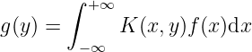
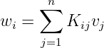
Integral transformation: function $f \overset{Integral}{\to}$ function $g$ where

∫ +∞ g(y) = −∞ K (x,y )f (x)dx

where $K (x, y)$ is called the kernal of the integral transformation. Analogy. Assuming $f$ is discrete, i.e.

f −→ v =, v(k ) = xk, k ∈ {1,...,n}

Similarly,

K (x, y) − → Kij, g − → w

then we have

∑n wi = Kijvj j=1

So integral transformation is the extension of linear transformation from finite dimension to infinite dimension.

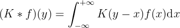
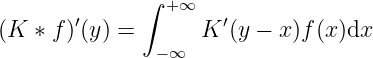
Particularly, if $K (x, y)$ has a form of $K (y - x)$ , then

∫ +∞ (K ∗ f)(y) = K (y − x )f (x)dx −∞

is called the convolution of $K$ and $f$ . At this time

∫ +∞ (K ∗ f)′(y) = K ′(y − x)f(x)dx −∞

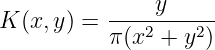
Example 3.4.1 The boundary value problem of Laplace function. Assuming $Ω = {(x, y) | y > 0} \subseteq R^{2}$ , then

\text{[math]}

Assuming

----y------ K (x, y) = π(x2 + y2)

we can verify that

$\int_{- \infty}^{+ \infty} K (x, y) d x = 1$ .
$\frac{\partial K}{\partial x} (x, y) = \frac{\partial K}{\partial y} (x, y)$ .
$Δ K = 0$ .

Assuming $f$ is continuous and bounded (within $M$ ), let

∫ ∫ +∞ y +∞ u(x,y ) = π-[(x-−-t)2 +-y2]f (t)dt = K (x − t,y)f(t)dt −∞ −∞

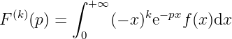
Then we have $\begin{aligned} Δ u & = \int_{- \infty}^{+ \infty} Δ K (x - t, y) f (t) d t = 0 \\ | u (x, y) - f (x) | & = | \int_{- \infty}^{+ \infty} \frac{y}{π [(x - t)^{2} + y^{2}]} (f (t) - f (x)) d t | \\ \leq \frac{1}{π} \int_{| t - x | < δ} \frac{y | f (t) - f (x) |}{π [(x - t)^{2} + y^{2}]} d t + \frac{1}{π} \int_{| t - x | \geq δ} \frac{y | f (t) - f (x) |}{π [(x - t)^{2} + y^{2}]} d t \\ \leq \frac{1}{π} \int_{| t - x | < δ} \frac{y ϵ}{π [(x - t)^{2} + y^{2}]} d t + \frac{1}{π} \int_{| t - x | \geq δ} \frac{y \cdot 2 M}{π [(x - t)^{2} + y^{2}]} d t \\ = ϵ + \frac{4 M}{π} (\frac{π}{2} - \arctan \frac{δ}{y}) \\ \Rightarrow | lim_{y \to + \infty} u (x, y) - f (x) | \leq 0 \Rightarrow lim_{y \to + \infty} u (x, y) = f (x) \end{aligned}$

Laplacian transformation.

∫ +∞ − px ℒ[f](p) = e f(x)dx = F (p) 0

If $\exists M > 0$ such that $\forall x > 0$ , $| f (x) | \leq M e^{α x}$ , then the Laplacian transformation exists when $p > a$ and $F \in C^{\infty}$ (Note: maybe $f$ is only integrable!). We can prove that

∫ +∞ F (k)(p) = (− x)ke−pxf(x)dx 0

Consider $\begin{aligned} L [f^{'}] (p) & = \int_{0}^{+ \infty} e^{- p x} f^{'} (x) d x = \int_{0}^{+ \infty} e^{- p x} d f (x) \\ = {e^{- p x} f (x) |}_{0}^{+ \infty} + p \int_{0}^{+ \infty} e^{- p x} f (x) d x = - f (0) + p L [f] (p) \end{aligned}$

So we have

\text{[math]}