Curve integral of the second kind

4.5 Curve integral of the second kind

Object being integrated: concerning vector field.
Geometric object carrying integration: oriented curve and surface.

Definition 4.5.1 Directional curve (path). Given $x : [a, b] \to Ω$ (a kind of motion), $x (t)$ represents the position ( $t$ is the time), $γ = {x (t) | t \in [a, b]}$ .

Note $x (t)$ is not a parametric representative of $γ$ ! Curve $γ$ is a static geometric object, while path $x (t)$ is a dynamic motion (meaning it could turn back along $γ$ ).

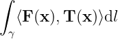
Example 4.5.1 Work done by force. $F (x) : Ω \to R^{m}$ (continuous) is a vector field where $x$ represents the position. Work

∫ ∫ b ′ ∫ x ′(t) ′ ∫ W = F ⋅ dx = ⟨F (x(t)),x (t)⟩dt = ∖lef t⟨F, ---′---∖right ⟩∥x (t)∥dt = ⟨F, T ⟩dl γ a γ ∥x (t)∥ γ

where $T (x)$ represents a forward-direction unit tangent vector field of $γ$ .

Flow velocity field $F$ (continuous). Assuming $T (x)$ represents a forward-direction unit tangent vector field of closed curve $γ$ , then the circulation is

∫ ⟨F(x ),T(x )⟩dl γ

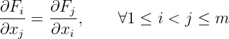
Assuming

F (x) =, x(t) =,a ≤ t ≤ b

Then we have

∫ ∫ ∫ b ∫ ′ ′ γ⟨F, T ⟩dl = γ F ⋅ dx = a [F1(x (t))x1(t) + ⋅⋅⋅ + Fm (x(t))x m(t)]dt = γ ω

where $ω = F_{1} (x) d x_{1} + \dots + F_{m} (x) d x_{m}$ has the form of first-order derivative.

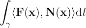
Example 4.5.2 Assuming $γ$ is a simple closed curve in plain (boundary of plain), $N (x)$ represents a forward-direction unit outer-norm vector field of $γ$ , then the flux is

∫ γ⟨F(x ),N (x )⟩dl

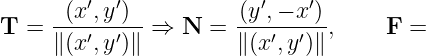
The relation between circulation and flux. Assuming the norm vector $k$ of the plain (direction determined by the forward direction of $γ$ and right-hand rule), then construct $\tilde{F} = k \times F$ where $\tilde{F}$ is derived by rotating $F$ by $90^{\circ}$ counterclockwise. Since $N = T \times k$ , naturally we have

∫ ∫ ∫ ∫ ⟨F, N ⟩dl = ⟨F, T × k ⟩dl = ⟨k × F, T⟩dl = ⟨F˜, T ⟩dl γ γ γ γ

Assuming

(x′,y ′) (y′,− x′) T = ---′--′--⇒ N = ---′--′--, F = ∥(x,y )∥ ∥(x ,y )∥

then we have

∫ ∫ ∫ b ′ ′ ⟨F,N ⟩dl = [X (x(t))y(t) − Y(x (t))x (t)]dt = (− Y dx + Xdy ) γ a γ

It also has a form of first-order derivative.

Example 4.5.3 Assuming

γ :

and its direction is determined by right-hand rule circling around $+ z$ axis. Seek $\int_{γ} z d x + x d y + y d z$ .

Firstly, seek the parametric equation of $γ$ . Eliminate $z$ by $z = - x - y$ to get $x^{2} + y^{2} + (- x - y)^{2} = R^{2}$ , so

y 2 3 2 R2 ∖left(x + -∖right ) + --y = --- 2 4 2

Let $(x + \frac{y}{2}, \frac{\sqrt{3}}{2} y) = \frac{R}{\sqrt{2}} (\cos θ, \sin θ)$ , then $z = - x - y = \dots$ .

The range of $θ$ . It is trivial that $θ \in [0, 2 π]$ .
Is the increasing direction of $θ$ the same as the direction of $γ$ ? Take $θ = 0$ , we can get that $(x, y) = (\frac{R}{\sqrt{2}}, 0)$ and $x^{'} < 0, y^{'} > 0$ . Then we can verify that these directions are the same.

Then on $γ$ , we have $\begin{aligned} ω & = (- x - y) d x + x d y + y d (- x - y) = - x d x - 2 y d x + x d y - y d y \\ = d (- \frac{x^{2}}{2} - \frac{y^{2}}{2} + x y) - 3 y d x \\ \int ω & = \underset{0 due to the closure of γ}{\underset{⏟}{\int_{γ} d (- \frac{x^{2}}{2} - \frac{y^{2}}{2} + x y)}} - \int_{γ} 3 y d x = - 3 \int_{γ} y d x \end{aligned}$

Then it’s left as exercise. :)

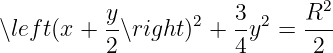
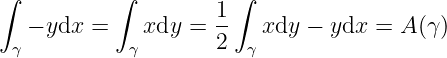
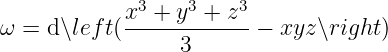
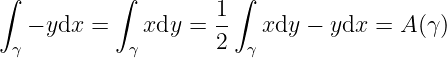
Example 4.5.4 Assuming $γ$ is a simple closed (Jordan) oriented (counterclockwise, natural positive direction) plain curve of $C^{1}$ , then

∫ ∫ ∫ − ydx = xdy = 1- xdy − ydx = A(γ ) γ γ 2 γ

where $A (γ)$ represents the area of closed domain bounded with $γ$ .

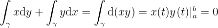
Assuming $(x (t), y (t)) = (r (t) \cos θ (t), r (t) \sin θ (t)), t \in [a, b]$ where $(x (a), y (a)) = (x (b), y (b))$ , then we have

∫ ∫ ∫ b xdy + ydx = d(xy) = x(t)y(t)|a = 0 γ γ γ

Notice that $\begin{aligned} \frac{1}{2} (x d y - y d x) & = \frac{1}{2} r (t) \cos θ (t) d (r (t) \sin θ (t)) - \frac{1}{2} r (t) \sin θ (t) d (r (t) \cos θ (t)) = r^{2} (t) θ^{'} (t) \\ \int_{γ} \frac{1}{2} (x d y - y d x) & = \frac{1}{2} \int_{a}^{b} r^{2} (t) θ^{'} (t) d t \end{aligned}$

So the former 2 equalities are proved.

Assuming $θ^{'} (t) \neq 0$ , then $θ (t)$ has inverse function $t (θ)$ , we have

∫ ∫ ∫ ∫ ∫ 1 1 b 2 1 b 2 2π r(𝜃) -(xdy − ydx ) = -- r (t(𝜃))d𝜃 = -- r (𝜃)d𝜃 = rdrd𝜃 = A (γ) γ 2 2 a 2 a 0 0

Theorem is proved.

Definition 4.5.2 $F : Ω \to R^{m}$ is a field with potential if $\exists f : Ω \to R$ such that $\forall x \in Ω$ , $F (x) = \nabla f (x)$ . $f$ is called a potential function of $F$ .

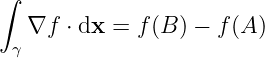
Theorem 4.5.3 For any path $γ$ (starting from $A$ , ending at $B$ ) of $C^{1}$ in $Ω$ , we have

∫ ∇f ⋅ dx = f (B) − f(A ) γ

Assuming

F == ∇f =

then we have

∂f ∂f ω = F1 (x )dx1 + ⋅⋅⋅ + Fm (x)dxm = ---dx1 + ⋅⋅⋅ +----dxm = df ∂x1 ∂xm

where $ω$ is called the total differential of $f$ . Then $\int_{γ} d f = f |_{A}^{B}$ (Newton-Leibniz formula).

Definition 4.5.4 If the integral of a vector field on any path only relates to the starting point and the destination, i.e. it has nothing to do with the path itself, then the vector field is conservative.

Corollary 4.5.5 Field with potential is conservative.

Theorem 4.5.6 Assuming $ω \subseteq R^{m}$ is a connected open set (domain), then any conservative field on $Ω$ has potential function.

Proof Mark $F$ as the conservative field, assuming $γ$ is a path from $A_{0}$ to $B (x)$ . Mark $f (x) = \int_{γ} F \cdot d x$ , it is to be proven that $\frac{\partial f}{\partial x_{1}} = F_{1} (x)$ .

Notice that $\begin{aligned} f (x + t e_{1}) - f (x) & = \int_{0}^{t} F (x + s e_{1}) \cdot \frac{d}{d s} (x + s e_{1}) d s = \int_{0}^{t} F (x + s e_{1}) \cdot e_{1} d s \\ = \int_{0}^{t} F_{1} (x + s e_{1}) d s \\ \frac{\partial f}{\partial x_{1}} (x) & = {\frac{d}{d t} f (x + t e_{1}) |}_{t = 0} = {F_{1} (x + t e_{1}) |}_{t = 0} = F_{1} (x) \end{aligned}$

Repeat this process, we can get that $\nabla f = F$ . $◻$

Example 4.5.5 Assuming $F (x) = - \frac{x}{∥ x ∥^{3}}$ , seek its potential function.

Notice that

2 ω = − --x1-dx1 − ⋅⋅⋅ − -xm--dxm = − d(∥x∥--)= − d∥x∥-= d--1-- ∥x ∥3 ∥x ∥3 2∥x∥3 ∥x∥2 ∥x ∥2

hence $f (x) = \frac{1}{∥ x ∥} + C$ .

Example 4.5.6 Seek

∫ y y (e + sinx )dx + (xe − cosy)dy γ

where $γ$ is part of $(x - π)^{2} + y^{2} = π^{2}$ , circling from $(0, 0)$ to $(π, π)$ in counterclockwise direction.

Notice that

ω = d(− cosx − sin y + xey)

hence

∫ ω = (− cos x − sin y + xey)|(π,π)= ⋅⋅⋅ γ (0,0)

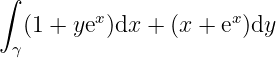
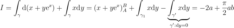
Example 4.5.7 Seek

∫ (x2 − yz)dx + (y2 − zx )dy + (z2 − xy )dz γ

where $γ : x = a \cos t, y = a \sin t, z = b t$ , $t \in [0, 2 π]$ , $a, b > 0$ .

Notice that

x3-+-y3-+-z3 ω = d∖left( 3 − xyz ∖right)

hence

∫ x3-+-y3 +-z3 2π ω = ∖left.∖left( 3 − xyz∖right)∖right |t=0 = ⋅⋅⋅ γ

Assuming

ω = F_{1} (x) d x_{1} + \dots + F_{m} (x) d x_{m} = d f

(

F = \nabla f

), then

F_{i} = \frac{\partial f}{\partial i}

. Assuming

f \in C^{2}

, we have

\frac{\partial^{2} f}{\partial x_{j} \partial x_{i}} = \frac{\partial^{2} f}{\partial x_{i} \partial x_{j}}

Definition 4.5.7 Assuming $F$ is a vector field. If

∂Fi- ∂Fj- ∂x = ∂x , ∀1 ≤ i < j ≤ m j i

then $F$ is irrotational.

Corollary 4.5.8 Conservative field is irrotational.

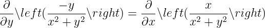
Example 4.5.8 Irrotational may not be conservative. Assuming $F = (\frac{- y}{x^{2} + y^{2}}, \frac{x}{x^{2} + y^{2}})^{T}$ is defined on $R^{2} ∖ {0, 0}$ , it is trivial that it is irrotational since

-∂- --−-y--- ∂-- --x----- ∂y ∖left(x2 + y2∖right ) = ∂x∖lef t( x2 + y2∖right)

Yet after transformation $(x, y) \to (r, θ)$ ,

∫ ∫ 2π ω = d𝜃 = 2π ⁄= 0 ∂B(0,a) 0

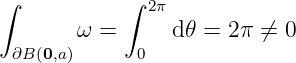
In fact, the integral reflects the geometric property of $γ$ – how many turns does $γ$ circle around the origin by.

Assuming $θ = \arctan \frac{y}{x}$ where $- \frac{π}{2} < θ < \frac{π}{2}$ , then

y- − ydx-+-xdy- y- d arctan x = x2 + y2 = ω, ∇ ∖lef t(arctan x ∖right) = F

Since we can’t define a singular-value continuous function $θ : R^{2} \to R$ , so the vector field above is not conservative! If the domain of definition $Ω : R^{2} ∖ {(x, 0) | x \geq 0}$ , then the vector field is conservative. It relates to the topological structure of the domain.

Plain vector field.

Physics: circulation – rotation, flux – divergence.
Mathematical form.

Definition 4.5.9 Assuming $F = (X, Y)^{T}$ is a vector field of $C^{1}$ , mark

∂Y ∂X ∂X ∂Y rotF = ----− ---, div F = ----+ ---- ∂x ∂y ∂x ∂x

respectively as the rotation and divergence of $F$ .

Theorem 4.5.10 (Green formula in physical form) Assuming $Ω \subseteq R^{2}$ is a bounded closed domain, $\partial Ω$ is piecewisely of $C^{1}$ , $F : Ω \to R^{2}$ is a vector field of $C^{1}$ , then

1.: $\int_{\partial Ω} F \cdot d x = \int_{Ω} rot F d x d y$ .
2.: $\int_{\partial Ω} ⟨ F, n ⟩ d l = \int_{Ω} div F d x d y$ .

where the forward direction of $\partial Ω$ is the natual positive direction.

Mark

\nabla = (\frac{\partial}{\partial x}, \frac{\partial}{\partial y}, \frac{\partial}{\partial z})

, we could mark

rot F = ∇ × F, div F = ∇ ⋅ F

Notice that

divF = tr ∂(X,-Y-) ∂(x,y)

indicating that the divergence has nothing to do with the selection of the coordinate system, since the similarity transformation of a matrix doesn’t change its trace.

Definition 4.5.11 Wedge (exterior) product. Define a formal product $d x \land d y$ satisfying

Binary linearity.
$(adx + bdx ) ∧ dy = adx ∧ dy + bdx ∧ dy 1 2 1 2$
Anti-symmetry.
$dx ∧ dy = − dy ∧ dx$

It is trivial that

d x \land d x = 0

. Actually,

d x \land d y

represents a oriented area, yet

d x d y

represents a non-oriented area. When moving forward along

\partial Ω

, the outside of

Ω

is on the right, i.e. the forward direction of

\partial Ω

is the natual positive direction, we have

d x \land d y = d x d y

Definition 4.5.12 Exterior differential. Assuming a form of first-order derivative $ω = X d x + Y d y$ , define

dω = dX ∧ dx + dY ∧ dy = ∖lef t(∂Y--− ∂X--∖right)dx ∧ dy ∂x ∂y

Then the third form of Green formula is

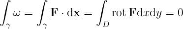
Theorem 4.5.13 (Green formula in mathematical form) $\int_{\partial Ω} ω = \int_{Ω} d ω$ .

Notice that

⟨F, n⟩dl = − Y dx + XdY = ˜ω

so we have

∂X ∂Y d˜ω = ∖lef t(∂x--+ -∂y-∖right)dx ∧ dy

verifying the second form of Green formula.

Note The physical meaning of divergence. Assuming $F$ is a vector field of $C^{1}$ , $Ω (ϵ) = B (P_{0}, ϵ)$ , then we have

∫ ∫ divF (P0) = lim -1-- div Fdxdy = lim -1-- ⟨F, n⟩dl 𝜖→0 π𝜖2 Ω 𝜖→0 π𝜖2 ∂Ω

Note

If $div F = 0$ , $F$ is called a non-source vector field.
If $rot F = 0$ , $F$ is called a irrotational field.
For a linear vector field $F (x) = A x$ , $tr A = 0 \Rightarrow F$ is non-source, $A$ is symmetric $\Leftrightarrow F$ is irrotational.

Corollary 4.5.14 If $Ω \subseteq R^{2}$ is a single-connected domain, i.e. any continuous closed loop in $Ω$ could become a single point after continuous transformation in $Ω$ , then any irrotational vector field of $C^{1}$ on $Ω$ is conservative.

Proof Assuming $D \subseteq Ω$ , $γ = \partial D$ is a closed loop, then we have

∫ ∫ ∫ ω = F ⋅ dx = rotFdxdy = 0 γ γ D

meaning $F$ is conservative. $◻$

Example 4.5.9 Prove

∫ ∫ 1 ∫ − ydx = xdy = -- xdy − ydx = A(γ ) γ γ 2 γ

with Green formula.

Assuming $ω_{1} = - y d x$ , then we have

∫ ∫ ∫ ∫ ∫ ω = dω = (− 1)dy ∧ dx = dx ∧ dy = dxdy = A(γ ) γ 1 D 1 D D D

Then it’s left as exercise. :)

Example 4.5.10 Assuming $γ : \frac{x^{2}}{a^{2}} + \frac{y^{2}}{b^{2}} = 1 (y \geq 0)$ from $A (a, 0)$ to $B (- a, 0)$ , seek

∫ (1 + yex)dx + (x + ex)dy γ

Let $γ^{'} : {(x, 0) | - a \leq x \leq a}$ from $B$ to $A$ , $γ_{1} = γ \cup γ^{'}$ is a closed loop. Notice that

∫ x ∫ x B ∫ ∫ π I = d (x + ye ) + xdy = (x + ye )A + xdy − xdy = − 2a + -ab γ γ γ1 ◟γ′◝◜--◞ 2 γ′:dy=0