Convergence of Fourier series

5.6 Convergence of Fourier series

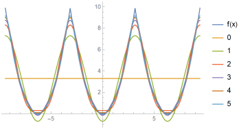
Figure 5.4 shows periodic function $f$ with period $2 π$ and its partial sum sequence of Fourier series.

Figure 5.4: $f (x) = x^{2}, x \in [- π, π]$ and its Fourier series

Theorem 5.6.1 (Pointwisely convergence) Assuming $f$ is piecewisely continuous and piecewisely derivable; and $\forall$ jump discontinuity $x_{0}$ of $f$ , $f^{'} (x_{0}^{+}), f^{'} (x_{0}^{-})$ is finite, then $\forall x$ , its Fourier series $S$ is convergent, and $S (x) = \frac{f (x^{+}) + f (x^{-})}{2}$

Definition 5.6.2 The inner product of 2 functions in $R [- π, π]$ is defined as $⟨ f, g ⟩ = \int_{- π}^{π} f (x) g (x) d x$ The $L^{2}$ -norm is defined as $∥ f ∥_{L^{2}} = ⟨ f, f ⟩ = \int_{- π}^{π} | f (x) |^{2} d x$

Definition 5.6.3 (Convergence in the mean square) If $∥ f_{n} - f ∥_{L^{2}} \to 0$ when $n \to + \infty$ , then $f_{n}$ converges to $f$ in the mean square, marked as $f_{n} \overset{L^{2}}{\to} f$ .

Theorem 5.6.4 (Least square property) Assuming $S_{N} = \frac{A_{0}}{2} + \sum_{n = 1}^{N} (A_{n} \cos n x + B_{n} \sin n x)$ is the partial sum of Fourier series of $f$ , mark $W_{N} = {\frac{α_{0}}{2} + \sum_{n = 1}^{N} (α_{n} \cos n x + β_{n} \sin n x) | α_{0}, α_{n} β_{n} \in R}$ then $L_{2 π}^{2} [- π, π] = {Periodic square-integrable function with period 2 π}$ is a infinite-dimension linear space, $W_{N} \subset L^{2}$ is the linear subspace and $\dim W_{N} = 2 N + 1$ . Assuming $T^{*}$ satisfies $min_{T \in W_{N}} ∥ f - T ∥ = ∥ f - T^{*} ∥$ then $T^{*} = S_{N}$ .

Proof Notice that $S_{N} = T^{*} \Leftrightarrow (f - S_{N}) ⊥ S_{N} \Leftrightarrow (f - S_{N}) ⊥ {1, \cos n x, \sin n x | 1 \leq n \leq N}$ Since $\begin{aligned} ⟨ f - T, 1 ⟩ & = ⟨ f, 1 ⟩ - ⟨ T, 1 ⟩ = π A_{0} - π α_{0} = 0 \Leftrightarrow A_{0} = α_{0} \\ ⟨ f - T, \cos n x ⟩ & = ⟨ f, \cos n x ⟩ - ⟨ T, \cos n x ⟩ = π A_{n} - π α_{n} = 0 \Leftrightarrow A_{n} = α_{n} \end{aligned}$

Similarly we have $B_{n} = β_{n}$ . So $S_{N} = T^{*}$ . $◻$

Corollary 5.6.5 (Bessel inequality) $π (\frac{A_{0}^{2}}{2} + \sum_{n = 1}^{N} (A_{n}^{2} + B_{n}^{2})) \leq \int_{- π}^{π} | f (x) |^{2} d x$

Proof Notice that $\begin{aligned} ∥ f ∥_{L^{2}}^{2} & = ∥ f - S_{N} ∥^{2} + ∥ S_{N} ∥^{2} \geq ∥ S_{N} ∥^{2} = {‖ \frac{A_{0}}{2} + \sum_{n = 1}^{N} (A_{n} \cos n x + B_{n} \sin n x) ‖}^{2} \\ = \frac{A_{0}^{2}}{4} ⟨ 1, 1 ⟩ + \sum_{n = 1}^{N} (A_{n}^{2} ⟨ \cos n x, \cos n x ⟩ + B_{n}^{2} ⟨ \sin n x, \sin n x ⟩) \end{aligned}$

So Bessel inequality is proved. $◻$

Corollary 5.6.6 Series $π (\frac{A_{0}^{2}}{2} + \sum_{n = 1}^{+ \infty} (A_{n}^{2} + B_{n}^{2}))$ is convergent, and $π (\frac{A_{0}^{2}}{2} + \sum_{n = 1}^{+ \infty} (A_{n}^{2} + B_{n}^{2})) \leq \int_{- π}^{π} | f (x) |^{2} d x$ This could be used to judge if a trignometric series is a Fourier series.

Corollary 5.6.7 (Parseval’s identity) Notice that $S_{N} \overset{L^{2}}{\to} f \Leftrightarrow ∥ S_{N} - f ∥_{L^{2}} \to 0 \Leftrightarrow ∥ S_{N} ∥_{L^{2}} \to ∥ f ∥_{L^{2}}$ we have $S_{N} \overset{L^{2}}{\to} f \Leftrightarrow π (\frac{A_{0}^{2}}{2} + \sum_{n = 1}^{+ \infty} (A_{n}^{2} + B_{n}^{2})) = \int_{- π}^{π} | f (x) |^{2} d x$

Theorem 5.6.8 For any $f \in L^{2}$ , Parseval’s identity holds.

Corollary 5.6.9 For any $f \in L^{2}$ , $S_{N} \overset{L^{2}}{\to} f$ .

Corollary 5.6.10 Assuming $f (x) = \frac{A_{0}}{2} + \sum_{n = 1}^{+ \infty} (A_{n} \cos n x + B_{n} \sin n x)$ and $g (x) = \frac{α_{0}}{2} + \sum_{n = 1}^{+ \infty} (α_{n} \cos n x + β_{n} \sin n x)$ , then $⟨ f, g ⟩ = π [\frac{A_{0} α_{0}}{2} + \sum_{n = 1}^{+ \infty} (A_{n} α_{n} + B_{n} β_{n})]$

We can use this to compute Riemann-

ζ

function. Define

ζ (z) = \sum_{n = 1}^{+ \infty} \frac{1}{n^{z}}

, we have

ζ (2) = \frac{π^{2}}{6}

ζ (4) = \frac{π^{4}}{90}

, ...

Applications of Fourier series.

Example 5.6.1 Isoperimetric inequality. Given a closed curve $γ$ where its length is $L$ and the area of its interior is $A$ . Assuming its parametric representative is $x, y : [0, L] \to R$ where $t \in [0, L]$ is the arc-length parameter and $x, y \in C^{2} [0, L]$ is periodic with period $L$ , then we have $4 π A \leq L^{2}$ where it takes the equality if and only if $γ$ is a circle.

Assuming $\begin{aligned} x (t) & = \frac{A_{0}}{2} + \sum_{n = 1}^{+ \infty} (A_{n} \cos \frac{2 n π t}{L} + B_{n} \sin \frac{2 n π t}{L}) \\ y (t) & = \frac{α_{0}}{2} + \sum_{n = 1}^{+ \infty} (α_{n} \cos \frac{2 n π t}{L} + β_{n} \sin \frac{2 n π t}{L}) \\ x^{'} (t) & = \sum_{n = 1}^{+ \infty} (- \frac{2 n π}{L} A_{n} \sin \frac{2 n π t}{L} + \frac{2 n π}{L} B_{n} \cos \frac{2 n π t}{L}) \\ y^{'} (t) & = \sum_{n = 1}^{+ \infty} (- \frac{2 n π}{L} α_{n} \sin \frac{2 n π t}{L} + \frac{2 n π}{L} β_{n} \cos \frac{2 n π t}{L}) \end{aligned}$

Since $t$ is the arc-length parameter, we have $x^{'} (t)^{2} + y^{'} (t)^{2} = 1$ . Then we have $\begin{aligned} L^{2} & = L \int_{0}^{L} (x^{'} (t)^{2} + y^{'} (t)^{2}) d t = L (⟨ x^{'}, x^{'} ⟩ + ⟨ y^{'}, y^{'} ⟩) \\ = L [\frac{L}{2} \frac{4 π^{2}}{L^{2}} \sum_{n = 1}^{+ \infty} n^{2} (A_{n}^{2} + B_{n}^{2}) + \frac{L}{2} \frac{4 π^{2}}{L^{2}} \sum_{n = 1}^{+ \infty} n^{2} (α_{n}^{2} + β_{n}^{2})] \\ = 2 π^{2} \sum_{n = 1}^{+ \infty} n^{2} (A_{n}^{2} + B_{n}^{2} + α_{n}^{2} + β_{n}^{2}) \\ A & = \frac{1}{2} \oint (- y d x + x d y) = \frac{1}{2} \int_{0}^{L} (- y (t) x^{'} (t) + x (t) y^{'} (t)) d t \\ = \frac{1}{2} (- ⟨ y, x^{'} ⟩ + ⟨ x, y^{'} ⟩) = π \sum_{n = 1}^{+ \infty} n (- α_{n} B_{n} + A_{n} β_{n}) \end{aligned}$

Notice that $L^{2} \geq 2 π^{2} \sum_{n = 1}^{+ \infty} n (B_{n}^{2} + α_{n}^{2} + A_{n}^{2} + β_{n}^{2}) \geq 4 π^{2} \sum_{n = 1}^{+ \infty} n (- α_{n} B_{n} + A_{n} β_{n}) = A$ Takes the equality.

$\forall n \geq 2$ , $A_{n} = B_{n} = α_{n} = β_{n} = 0$ .
$\forall n \in N^{*}$ , $A_{n} = β_{n}$ , $α_{n} = - B_{n}$ .

Therefore, ${\begin{cases} x (t) = \frac{A_{0}}{2} + A_{1} \cos \frac{2 π t}{L} + B_{1} \sin \frac{2 π t}{L} \\ y (t) = \frac{α_{0}}{2} - B_{1} \cos \frac{2 π t}{L} + A_{1} \sin \frac{2 π t}{L} \end{cases} \Rightarrow {(x - \frac{A_{0}}{2})}^{2} + {(y - \frac{α_{0}}{2})}^{2} = A_{1}^{2} + B_{1}^{2}$ meaning it’s a circle.

Example 5.6.2 Seek the periodic solution with period $2 π$ to $y^{″} + λ y = \sin x$ , i.e. ${\begin{cases} y^{″} + λ y = \sin x \\ y (0) = y (2 π) \\ y^{'} (0) = y^{'} (2 π) \end{cases}$ This is called the boundary problem.

Assuming $y (x) = \frac{A_{0}}{2} + \sum_{n = 1}^{+ \infty} (A_{n} \cos n x + B_{n} \sin n x)$ , then $y^{″} (x) = - \sum_{n = 1}^{+ \infty} n^{2} (A_{n} \cos n x + B_{n} \sin n x)$ After substitution, we have

Constant term. $λ \frac{A_{0}}{2} = 0$ .
$\cos n x$ term. $- n^{2} A_{n} + λ A_{n} = 0$ .
$\sin n x$ term. $- n^{2} B_{n} + λ B_{n} = δ_{n 1}$ .

Discussion on $λ$ .

When $λ = 0$ , then $A_{0}$ is arbitrary; $A_{n} = 0$ , $\forall n \geq 1$ ; $B_{n} = - δ_{n 1}$ ; so $y (x) = \frac{A_{0}}{2} - \sin x$ are all periodic solutions with period $2 π$ . Infinite solution, dimension $= 1$ , affine space.
When $λ \neq n^{2} (n = 0, 1, . . .)$ , then $A_{n} = 0$ , $\forall n \geq 0$ ; $B_{n} = 0$ , $\forall n > 1$ ; $B_{1} = \frac{1}{λ - 1}$ ; so $y (x) = \frac{1}{λ - 1} \sin x$ is the unique periodic solution with period $2 π$ .
When $λ = 1$ , then $A_{0} = 0$ ; $A_{1}$ is arbitrary; $A_{n} = B_{n} = 0$ , $\forall n \geq 1$ ; yet $- B_{1} + B_{1} = 1$ is impossible; so there doesn’t exist a periodic solution with period $2 π$ .
When $λ = m^{2} (m > 1)$ , then $A_{n} = 0$ , $\forall n \neq m$ ; $A_{m}$ is arbitrary; $B_{1} = \frac{1}{m^{2} - 1}$ ; $B_{n} = 0$ , $\forall n \neq m$ and $n \neq 1$ ; $B_{m}$ is arbitrary; so $y (x) = \frac{\sin n x}{m^{2} - 1} + A_{m} \cos m x + B_{m} \sin m x$ are all periodic solutions with period $2 π$ . Infinite solution, dimension $= 2$ , affine space.

Assuming a linear transformation operator $L : L y = - y^{″}$ which operates on the linear space $V$ composed of all periodic functions with period $2 π$ , then the original equation could be rewritten as $- L y + λ y = \sin x$ Recall in linear algebra, given $x, b \in R^{n}$ and a square matrix $A \in M_{n}$ , for the equation $- A x + λ x = b \Leftrightarrow (λ I - A) x = b$ Assuming $λ$ is not the eigenvalue of $A$ , then $λ I - A$ is invertible, so $\forall b \in R^{n}$ , $(λ I - A) x = b$ has a unique solution.

Assuming $λ$ is the eigenvalue of $A$ , then $(λ I - A) x = b$ has a solution $\Leftrightarrow$ $b \in Im (λ I - A)$ . Assuming $A$ is symmetric, then we have $R^{n} = \ker (λ I - A) \underset{⊥}{\oplus} Im (λ I - A)$ Here $b \in Im (λ I - A) \Leftrightarrow b ⊥$ all eigenvectors of $A$ corresponded to eigenvalue $λ$ .

$L$ is symmetric since $⟨ L f, g ⟩ = ⟨ f, L g ⟩$ . $\forall f, g$ , i.e. $\begin{aligned} ⟨ L f, g ⟩ & = \int_{0}^{2 π} (- f^{″}) g d x = - \int_{0}^{2 π} g d f^{'} = - f^{'} g |_{0}^{2 π} + \int_{0}^{2 π} f^{'} g^{'} d x = \int_{0}^{2 π} f^{'} g^{'} d x \\ ⟨ f, L g ⟩ & = \int_{0}^{2 π} (- g^{″}) f d x = - \int_{0}^{2 π} f d g^{'} = - g^{'} f |_{0}^{2 π} + \int_{0}^{2 π} f^{'} g^{'} d x = \int_{0}^{2 π} f^{'} g^{'} d x \end{aligned}$

Assuming $λ$ is eigenvalue of $L$ , i.e. $(λ I - L) y = λ y + y^{″} = 0$ .

$λ < 0$ , only zero solution in $V$ , so $λ$ is not eigenvalue.
$λ = 0$ is the eigenvalue, $y \equiv 1$ is the base of eigen-subspace, $\dim = 1$ .
$λ > 0, λ \neq n^{2} (n = 1, 2, . . .)$ , only zero solution in $V$ , so $λ$ is not the eigenvalue.
$λ = n^{2}$ is the eigenvalue, $\cos n x, \sin n x$ are the bases of eigen-subspace, $\dim = 2$ .