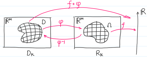
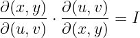
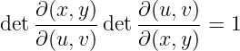
See Figure 4.2. Assuming where is a bounded closed and Jordan-measurable, ; is a diffeomorphism
of (invertible coordinate transformation of ) where is a bounded closed and Jordan-measurable, then
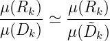
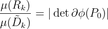
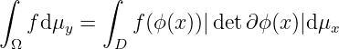
we can prove that
Therefore,
Figure 4.2: Change of variable for multiple integral
Example 4.3.1
1.
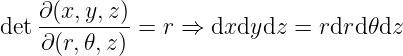
Polar coordinate (in 2-dimension).
2.
Cylindrical coordinate.
We have
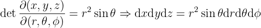
3.
Spherical coordinate.
We have
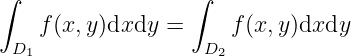
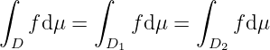
Symmetries of multiple integral. Assuming , and ; , , then we have
ProofFirstly,
For , we take a variable transformation:
then , we have
Note According to IFT,
Therefore,
Example 4.3.2, seek . Let
which is diffeomorphism of , then , so
Example 4.3.3, seek .
Take a polar transformation , we have where , then
It is not perfectly correct, since is unbounded near . It’s a multiple improper integral.
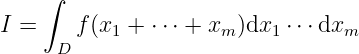
Example 4.3.4, seek
Take a variable transformation
then we have
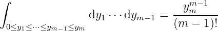
How to calculate the integral in ? Firstly,
Then, consider the order of . For any arrangement of ,
The determinant of a permutation matrix is either or , so
Notice that
Therefore
Terminally
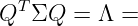
Example 4.3.5 Assuming , is a symmetric positive-definite matrix of -order, prove
that
According to spectral theorem, is symmetric and positive-definite, so there exists an orthogonal
matrix such that
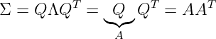
where . Then
where is invertible. Let , then where and are diffeomorphism, hence
Notice that
therefore
How to calculate the last integral? Consider
Terminally .
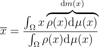
Center of mass. Assuming an object occupying , its mass distribution (density) is
The center of mass is defined as
It’s a weighted average.
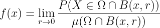
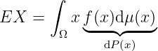
Another similar example is in probability theory. Assuming a random variable , the probability
density is defined as
The (mathematical) expectation is defined as
It’s also a weighted average.
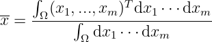
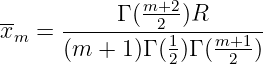
Example 4.3.6 Assuming , its mass is evenly distributed, i.e. . Seek the center of mass of
.
According to the definition, we have
Firstly,
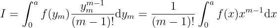
. Assuming where has nothing to do with (proven by mathematical induction), we have
Therefore,
According to symmetry,
As for , we have
Terminally,
Example 4.3.7 Select numbers at random in (independent and evenly distributed), seek the mean
value (expectation) of the minimum value.
The probability density is , the joint density of random numbers is
, then the expectation of the minimum value is
Example 4.3.8 Assuming the radius and density of a 3-dimension ball are respectively , seek its
gravitational force applied to a mass point outside the ball.
Construct the coordinate system where the center of the ball is put at origin and the mass point is
put at . For a point in the ball, we have
Therefore,
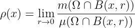
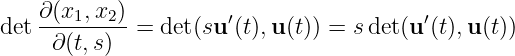
Example 4.3.9 Kepler II law for centripetal (centrifugal) force field. The motion of a mass point on
a plain where . Assuming is covered by a line connecting a planet to the sun over certain period of
time , let , we have
then the area of is
Kepler II:
By taking the derivative, we have
meaning are linear dependent, i.e. the force field is centripetal (centrifugal).


![∫
dy1 ⋅⋅⋅dym −1 = ymm− 1
y1,...,ym− 1∈[0,ym]](main261x.png)


![∫
------1------- 1- T −1
I = ℝm ∘ (2π )m detΣ exp ∖left[− 2(x − μ) Σ (x − μ )∖right ]dx1 ⋅⋅⋅dxm = 1](main266x.png)
![∫
1 1 T T − 1 ∂x
I = ∘------m------exp ∖lef t[− -y A Σ Ay ∖right ]∖left|det ---∖right|dy1⋅⋅⋅dym
ℝm (2 π) detΣ 2 ∂y](main269x.png)


![∫ ∫ ∫ b
A = dx1dx2 = ∖left|det ∂(x1,x2)∖right |dtds = 1- |det(u ′(t),u(t))|dt
Ω [a,b]× [0,1] ∂(t,s) 2 a](main282x.png)

![d-∖left[det(u′(t),u (t))∖right] = det(u′′(t),u(t)) + det(u ′(t),u′(t)) = det(u ′′(t),u (t)) = 0
dt](main284x.png)