Derivative of multiple variable function

2.1 Derivative of multiple variable function

In single variable function, the derivative of $f$ at $x = x_{0}$ is defined as

f (x ) − f (x0) f(x0 + h) − f(x0) f ′(x0) = lim -------------= lim ------------------ x→x0 x − x0 h→0 h

In multiple variable function, since one could not be divided by a vector, so we should rewrite the expression above. $\begin{aligned} \frac{f (x_{0} + h) - f (x_{0})}{h} - f^{'} (x_{0}) & \to 0 \\ \frac{f (x_{0} + h) - f (x_{0}) - f^{'} (x_{0}) h}{h} & \to 0 \\ \frac{∥ f (x_{0} + h) - f (x_{0}) - f^{'} (x_{0}) h ∥}{∥ h ∥} & \to 0 \end{aligned}$

Definition 2.1.1 $x_{0}$ is the interior point of $E \subseteq R^{m}$ if there exists $δ_{0} > 0$ such that $B (x_{0}, δ_{0}) = {x \in R^{m} | ∥ x - x_{0} ∥ < δ_{0}} \subseteq E$ . $B (x_{0}, δ_{0})$ is also called an $δ_{0}$ -open ball at $x_{0}$ .

Definition 2.1.2 $f : E \to R^{p}$ is derivable (differentiable) at $x_{0}$ if there exists a linear mapping $A : R^{m} \to R^{p}$ such that $f (x_{0} + h) = f (x_{0}) + A h + o (h)$ , $h \to 0$ . $A$ is called the derivative of $f$ at $x_{0}$ , marked as $A = \partial f (x_{0})$ or $D f (x_{0})$ .

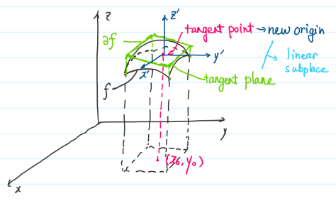
Note In 1-dimension case, the derivative $A = f^{'} (x_{0})$ is also a linear mapping, merely here the preimage space and the image space are both 1-dimension, so $A : R \to R$ is equivalent to the coefficient of the proportional function, reduced to a number. The geometric meaning of derivative is shown in Figure 2.1.

Figure 2.1: The geometric meaning of derivative

When $m = 1$ , $p \geq 1$ , consider the derivative of $f : (a, b) \to R^{p}$ at $t_{0} \in (a, b)$ . Traditionally,

′ f(t0 +-h-) −-f-(t0)- f (t0) = lhim→0 h

If regard $f$ as a kind of motion, then $f^{'} (t_{0})$ is the instantaneous velocity when $t = t_{0}$ .

′ f(t0 + h) = f◟(t0) +◝f◜-(t0)h◞ +o (h) uniform linear motion

is the best uniform linear motion to approximately describe the original real motion. Here $f^{'} (t_{0}) h = \partial f (t_{0}) (h)$ , it connects the derivative with the differential.

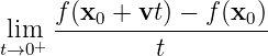
Definition 2.1.3 Given $E \subseteq R^{m}$ , $f : E \to R^{p}$ , $x_{0}$ is the interior point of $E$ . Then for any $v \in R^{m}$ , if

lim f(x0-+-vt)-−-f(x0-) t→0+ t

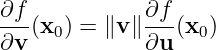
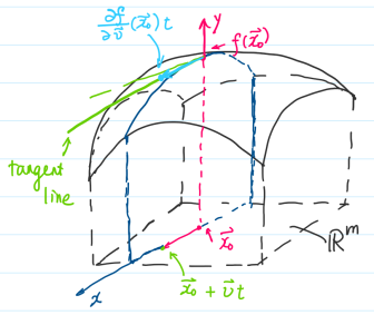
exists, then it’s marked as $\frac{\partial f}{\partial v} (x_{0})$ , called the derivative of $f$ along $v$ at $x_{0}$ . Particularly, if $∥ v ∥ = 1$ , then it’s called the directional derivative.

Note

Notice that $t \to 0^{+}$ ! When $t < 0$ , it’s a different directional derivative along $- v$ !
Mark $v = ∥ v ∥ u$ , then $\begin{aligned} \frac{\partial f}{\partial v} (x_{0}) & = lim_{t \to 0^{+}} \frac{f (x_{0} + v t) - f (x_{0})}{t} = ∥ v ∥ lim_{t \to 0^{+}} \frac{f (x_{0} + u ∥ v ∥ t) - f (x_{0})}{∥ v ∥ t} \\ \overset{t^{'} = ∥ v ∥ t}{\to} ∥ v ∥ lim_{t^{'} \to 0^{+}} \frac{f (x_{0} + u t^{'}) - f (x_{0})}{t^{'}} = ∥ v ∥ \frac{\partial f}{\partial u} (x_{0}) \end{aligned}$

Therefore for any $v$ ,
$∂f-(x ) = ∥v∥-∂f(x ) ∂v 0 ∂u 0$
The geometric meaning of directional derivative is shown in Figure 2.2. The slope of the green tangent line in $x O y$ plane (dark blue $x$ and magenta $y$ coordinate) is the directional derivative of $f$ along $v$ at $x_{0}$ .
If $f$ is derivable at $x_{0}$ , then the directional derivative along any direction exists; yet even the directional derivative along any direction exists, it might be even not continuous!

Figure 2.2: The geometric meaning of directional derivative

Theorem 2.1.4

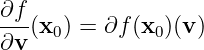
1.: If $f$ is derivable at $x_{0}$ , then for any $v \in R^{m}$ , $\frac{\partial f}{\partial v} (x_{0})$ exists where
$∂f ---(x0) = ∂f (x0)(v) ∂v$
2.: When $m \geq 2$ , there exists $f$ such that for any $v \in R^{m}$ , $\frac{\partial f}{\partial v} (x_{0})$ exists, yet $f$ is not continuous at $x_{0}$ . It is mainly because except for $m = 1$ , there are infinite directional derivatives (only $2$ when $m = 1$ ).

Example 2.1.1 Several examples for derivable functions.

1.

Constant mapping.

2.

Linear mapping.

3.

Inner product. Given a linear mapping $A$ , $f : R^{n} \to R^{n}$ where $f (x) = ⟨ A x, x ⟩$ is derivable at any $x_{0}$ . Notice that $\begin{aligned} f (x_{0} + h) & = ⟨ A (x_{0} + h), x_{0} + h ⟩ - ⟨ A x_{0}, x_{0} ⟩ \\ = ⟨ A x_{0}, h ⟩ + ⟨ A h, x_{0} ⟩ + ⟨ A h, h ⟩ \\ = \underset{linear with respect to h}{\underset{⏟}{⟨ A x_{0}, h ⟩ + ⟨ A h, x_{0} ⟩}} + O (∥ h ∥^{2}) \\ = ⟨ (A + A^{T}) x_{0}, h ⟩ + o (h) \end{aligned}$

4.

$A$ is a square matrix, $f (A) = A^{- 1}$ is derivable.

Consider $A = I$ first. For any $∥ B ∥ < 1$ , $I + B$ is invertible (proved in the homework). Notice that $\begin{aligned} (I + B) (I - B) & = I - B^{2} \\ (I + B) [I - B + (I + B)^{- 1} B^{2}] & = I \end{aligned}$

Therefore $f (I + B) = I - B + (I + B)^{- 1} B^{2}$ . Notice that $\begin{aligned} ∥ (I + B)^{- 1} B^{2} ∥ & \leq ∥ (I + B)^{- 1} ∥ ∥ B ∥^{2} \\ \leq [∥ (I + B)^{- 1} - I ∥ + ∥ I ∥] ∥ B ∥^{2} \\ \leq [\frac{∥ B ∥}{1 - ∥ B ∥} + 1] ∥ B ∥^{2} = \frac{∥ B ∥^{2}}{1 - ∥ B ∥} \\ \leq 2 ∥ B ∥^{2} = O (∥ B ∥^{2}) = o (B) \end{aligned}$

when $∥ B ∥ < \frac{1}{2}$ . So $f (I + B) = f (I) - B + o (∥ B ∥)$ , i.e. $\partial f (I) (B) = - B$ .

Consider invertible $A$ then. $A + B = A (I + A^{- 1} B)$ is invertible when $∥ A^{- 1} B ∥ < 1$ , i.e. $∥ B ∥ < \frac{1}{∥ A^{- 1} ∥}$ . So $f$ is derivable at $A$ . Notice that $\begin{aligned} f (A + B) & = (A + B)^{- 1} = (I + A^{- 1} B)^{- 1} A^{- 1} \\ = f (I + A^{- 1} B) A^{- 1} \\ = [f (I) - A^{- 1} B + o (B)] A^{- 1} \\ = A^{- 1} - A^{- 1} B A^{- 1} + o (B) \end{aligned}$

Therefore $\partial f (A) (B) = - A^{- 1} B A^{- 1}$ .

5.

If $F$ and $G$ are both derivable at $x_{0}$ , then $H (x) = ⟨ F (x), G (x) ⟩$ is derivable. Notive that $\begin{aligned} H (x_{0} + h) - H (x_{0}) \\ = ⟨ F (x_{0} + h), G (x_{0} + h) ⟩ - ⟨ F (x_{0}), G (x_{0}) ⟩ \\ = ⟨ F (x_{0}) + \partial F (x_{0}) (h) + o (h), G (x_{0}) + \partial G (x_{0}) (h) + o (h) ⟩ - ⟨ F (x_{0}), G (x_{0}) ⟩ \\ = \underset{linear with respect to h}{\underset{⏟}{⟨ F (x_{0}), \partial G (x_{0}) (h) ⟩ + ⟨ \partial F (x_{0}) (h), G (x_{0}) ⟩}} + o (h) \end{aligned}$

Therefore

∂H (x0)(h ) = ⟨F (x0),∂G (x0)(h )⟩ + ⟨∂F (x0)(h),G (x0)⟩

6.

Consider $det : M_{n} \to R$ , we have

∑ det (A ) = 𝜖σ ,...,σ A1 σ ⋅⋅⋅Anσ σ ,...,σ 1 n 1 n 1 n

where $ϵ_{σ_{1}, . . ., σ_{n}}$ is Levi-Civita symbol. Consider a mapping $e_{i j} : M_{n} \to R$ , $A \mapsto A_{i j}$ . It’s linear, so it’s differentiable. Since $det (A)$ is composed by the addition, multiplication and composition of $e_{i j}$ , all $e_{i j}$ are differentiable, therefore, $det (A)$ is differentiable.

Consider a special matrix $E_{i j}$ whose elements are all $0$ except that the row $i$ column $j$ element is $1$ . ${E_{i j}}$ compose a set of bases of $M_{n}$ . Notice that

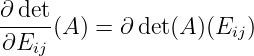
∂ det -----(A) = ∂ det(A )(Eij) ∂Eij

we have

∗ ∗ ∗ ∗ det(A + tEij) = a1jA1j + ⋅⋅⋅ + (aij + t)A ij + ⋅⋅⋅ + anjA nj = det(A ) + tA ij

i.e.

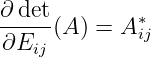
∂ det-(A) = A ∗ ∂Eij ij

Therefore $\begin{aligned} \partial det (A) (B) & = \partial det (A) (\sum_{i, j}^{n} b_{i j} E_{i j}) = \sum_{i, j}^{n} b_{i j} \frac{\partial det}{\partial E_{i j}} (A) \\ = \sum_{i j}^{n} b_{i j} A_{i j}^{*} = \sum_{j = 1}^{n} \sum_{i = 1}^{n} (A^{*})_{j i}^{T} b_{i j} \\ = \sum_{j = 1}^{n} (A^{* T} B)_{j j} = tr (A^{* T} B) \end{aligned}$

Terminally

det(A + B ) = det(A ) + tr(A ∗TB ) + o(B )

Theorem 2.1.5 Chain rule. Given $F : E \to R^{p}$ , $G : R^{p} \to R^{q}$ , $F$ is derivable at $x_{0}$ , $G$ is derivable at $y_{0} = F (x_{0})$ , then $G \circ F$ is derivable at $x_{0}$ where $\begin{aligned} \partial (G \circ F) (x_{0}) & = \partial G (y_{0}) \circ \partial F (x_{0}) \\ \partial (G \circ F) (x_{0}) (h) & = \partial G (y_{0}) (\partial F (x_{0}) (h)) \end{aligned}$

It’s called the differentiation of the composition is the composition of the differentiation.