Implicit function theorem

2.5 Implicit function theorem

Background. Implicit function theorem (IFT) is based on solving equations $F (X) = 0$ . They can be classified into $\begin{aligned} (1) Inverse mapping & F (\underset{unknown}{\underset{⏟}{x}}) = \underset{known}{\underset{⏟}{y}} & \overset{?}{\to} & x = G (y) \\ (2) Implicit function & F (\underset{known}{\underset{⏟}{x}}, \underset{unknown}{\underset{⏟}{y}}) = 0 & \overset{?}{\to} & y = G (x) \end{aligned}$

Does any solution exist?
How many solutions does it give?
The continuity, derivability of the solution over arguments?
(1),(2) are related, since $\tilde{F} (y, x) = F (x) - y = 0$ .
If $X, Y$ has the dimension, then there exists a method to transform an implicit function $F (X, Y) = 0$ into an inverse mapping $\tilde{F} (Y) = X$ .

Theorem 2.5.1 (IFT) Assuming $F : R^{m} \times R^{n} \to R^{n}$ , $F \in C^{k}$ subjecting to

$F (x_{0}, y_{0}) = 0$ .
$\partial_{y} F (x_{0}, y_{0})$ is invertible.

then there exists a neighborhood $U = V \times W$ near $(x_{0}, y_{0})$ and mapping $g : V \to W \in C^{k}$ such that for any $(x, y) \in U$ , $F (x, y) = 0 \Leftrightarrow y = g (x)$ .

Proof

1.

Linearize $F$ near $(x_{0}, y_{0})$ to get

F (x,y ) = F (x ,y ) + ∂ F(x ,y )(x − x ) + ∂ F (x ,y )(y − y ) + α(x,y ) 0 0 x 0 0 0 y 0 0 0

where $α (x, y) = o (∥ x - x_{0} + y - y_{0} ∥)$ . Since $F (x, y) = F (x_{0}, y_{0}) = 0$ , and for the solution to the linear function we let $α (x, y) = 0$ , therefore

y = y − (∂ F (x ,y ))− 1∂ F (x ,y )(x − x ) 0 y 0 0 x 0 0 0

It is the unique solution to the linear function. We hope the solution for the original function has a form of

−1 y = y0 − (∂yF (x0,y0)) ∂xF (x0,y0)(x − x0 ) + β (x )

where $β (x) = o (∥ x - x_{0} ∥)$ . If $g$ exists and $g$ is derivable, then take the derivative over $x$ of

F (x,g(x )) = 0 ∀x

we can get $\begin{array}{r} \partial_{x} F (x, g (x)) + \partial_{y} F (x, g (x)) \partial g (x) = 0 \\ \partial g (x) = - (\partial_{y} F (x, g (x)))^{- 1} \partial_{x} F (x, g (x)) \end{array}$

2.

Prove $g \in C^{k}$ by mathematical induction.

$F \in C^{1} \Rightarrow \partial_{y} F, \partial_{x} F \in C^{0}$ , therefore $\partial_{y} F (x, g (x)), \partial_{x} F (x, g (x))$ are both continuous. Since $A \mapsto A^{- 1}$ is infinitely derivable, so $\partial g \in C^{0}$ , meaning $g \in C^{1}$ .
$F \in C^{k + 1} \Rightarrow F \in C^{k} \Rightarrow g \in C^{k} \Rightarrow (\partial_{y} F (x, g (x)))^{- 1}, \partial_{x} F (x, g (x)) \in C^{k} \Rightarrow \partial g (x) \in C^{k} \Rightarrow g \in C^{k + 1}$ .

3.

If $g$ exists and is continuous, then $g$ is derivable. Notice that

0 = F (x,g(x)) = F (x0,y0) + ∂xF (x0,y0)(x − x0 ) + ∂yF (x0,y0 )(g (x ) − y0 ) + α (x,g(x))

For $α$ , $\forall ϵ > 0$ , there exists $δ_{ϵ} > 0$ such that

˜ ∥x − x0 ∥ < δ𝜖 < δ𝜖,∥g(x ) − y0 ∥ < δ𝜖 ⇒ ∥α (x,g(x))∥ ≤ 𝜖(∥x − x0 ∥ + ∥g (x) − y0∥)

where ${\tilde{δ}}_{ϵ}, δ_{ϵ}$ are related with the continuity of $g$ . Then

g(x) = y0 − (∂yF (x0,y0))−1∂xF (x0,y0 )(x − x0 ) − (∂yF (x0,y0 ))− 1α(x,g(x ))

$\begin{aligned} ∥ g (x) - y_{0} ∥ & = M_{1} ∥ x - x_{0} ∥ + M_{2} ϵ (∥ x - x_{0} ∥ + ∥ g (x) - y_{0} ∥) \\ \leq \frac{M_{1} ∥ x - x_{0} ∥ + M_{2} ϵ ∥ x - x_{0} ∥}{1 - M_{2} ϵ} \leq C ∥ x - x_{0} ∥ \end{aligned}$

$\begin{aligned} ∥ g (x) - y_{0} + (\partial_{y} F (x_{0}, y_{0}))^{- 1} \partial_{x} F (x_{0}, y_{0}) (x - x_{0}) ∥ & \leq M_{2} ϵ (∥ x - x_{0} ∥ + ∥ g (x) - y_{0} ∥) \\ \leq M_{2} (1 + C) ϵ ∥ x - x_{0} ∥ \end{aligned}$

4.

Proof 1 (with fixed point): Notice that

− 1 F (x, y) = 0 ⇔ G (x,y) = (∂yF (x0,y0 )) F (x,y ) = 0

where $G (x_{0}, y_{0})) = 0$ and $\partial_{y} G (x_{0}, y_{0}) = I$ .

Construct $T_{x} (y) = y - G (x, y)$ , then $G (x, y) = 0 \Leftrightarrow T_{x} (y) = y$ . Notice that

∂Tx0 (y0) = I − ∂yG (x0,y0) = 0

meaning $\partial T_{x} (y) \sim 0$ , i.e. $∥ \partial T_{x} (y) ∥ \leq \frac{1}{2}$ . $\dots \dots$

This proof doesn’t involve the dimension, meaning it holds for even infinite dimension.

5.

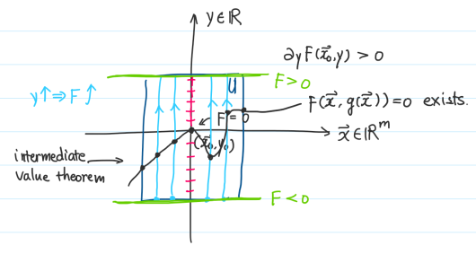
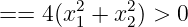
Proof 2 (finite dimension only): Proof by mathematical induction over the dimension $n$ . $F (x, y) = 0 \in R$ , $y \in R$ . $F (x_{0}, y_{0}) = 0$ , $\partial_{y} F (x_{0}, y_{0}) \in R^{*}$ . Assuming $\partial_{y} F (x_{0}, y_{0}) > 0$ , otherwise consider $- F$ . See proof hint in Figure 2.4. $◻$

Theorem 2.5.2 Inverse mapping theorem. Assuming $F : R^{n} \to R^{n} \in C^{k}$ , $\partial F (x_{0})$ is invertible, then there exists a neighborhood $U$ near $x_{0}$ , a neighborhood $V$ near $y_{0} = F (x_{0})$ and a unique mapping $G : U \to V \in C^{k}$ such that $G (F (x)) = x$ , $\forall x \in U$ .

Proof Assuming $H (x, y) = F (x) - y = 0$ , $H (x_{0}, y_{0}) = 0$ and $\partial_{x} H (x_{0}, y_{0}) = \partial_{x} F (x_{0})$ is invertible. From IFT, there exists a unique $G (y) = x$ such that $H (G (y), y) = 0$ , i.e. $F (G (y)) = y$ , hence $G (F (x)) = G (F (G (y))) = G (y) = x$ . $◻$

Example 2.5.1 For the matrix equation $X^{2} + t A X - I = 0$ , prove that when $t ≃ 0$ , there exists a unique solution $X (t) \in C^{\infty}$ where $X (0) = I$ . Find an approximate expression of $X (t)$ .

Construct $F (t, X) = X^{2} + t A X - I$ where $F (0, I) = 0$ , notice that, $\begin{aligned} F (t, I + B) & = (I + B)^{2} + t A (I + B) - I \\ = \underset{linear}{\underset{⏟}{t A + 2 B}} + \underset{o (| t | + ∥ B ∥)}{\underset{⏟}{B^{2} + t A B}} \end{aligned}$

meaning $\partial_{X} F (0, I) : M_{n} \to M_{n} = 2 B$ is invertible.

According to IFT, there exists $δ_{1} > 0, δ_{2} > 0$ such that $\forall | t | < δ_{1}$ , $\forall ∥ X - I ∥ < δ_{2}$ , $\exists g$ such that $F (t, X) = 0 \Leftrightarrow X = g (t) = X (t)$ . $F \in C^{\infty} \Rightarrow g \in C^{\infty}$ , meaning $X (t)$ is $C^{\infty}$ with respect to $t$ .

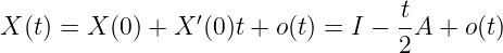
Therefore, for any $| t | < δ_{1}$ , $X (t)^{2} + t A X (t) - I = 0$ . Take the derivative over $t$ ,

X ′(t)X (t) + X (t)X ′(t) + AX (t) + tAX ′(t) = 0, ∀t

Take $t = 0$ , we have $X (0) = I$ , hence $X^{'} (0) = - \frac{A}{2}$ ,

t X (t) = X (0) + X ′(0 )t + o(t) = I − -A + o(t) 2

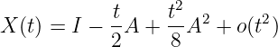
Take the second derivative over $t$ ,

′′ ′ 2 ′′ ′ ′′ X (t)X (t) + 2X (t) + X (t)X (t) + 2AX (t) + tAX (t) = 0, ∀t

Take $t = 0$ , we have $X (0) = I$ , $X^{'} (0) = - \frac{A}{2}$ , hence $X^{″} (0) = \frac{A^{2}}{4}$ ,

t t2 X (t) = I − -A + --A2 + o(t2) 2 8

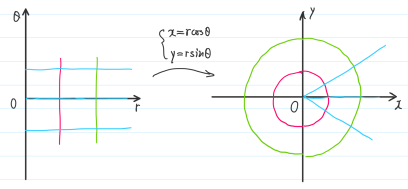
Example 2.5.2 Polar coordinate $(r, θ)$ and orthogonal coordinate $(x, y)$ , we have

\text{[math]}

The mapping above $f : (0, + \infty) \times (- \infty, \infty) \to R^{2} ∖ {(0, 0)} \in C^{\infty}$ . Consider its Jacobi matrix

=

It’s determinant is $r > 0$ , meaning its linearly invertible. According to IMT, there exists a local inverse mapping of $C^{\infty}$ .

Definition 2.5.3 Assuming $U, V$ are 2 open sets in $R^{n}$ . $F : U \to V$ is a diffeomorphism of $C^{k}$ if there exists an inverse mapping $F^{- 1} : V \to U$ of $F$ and $F^{- 1} \in C^{k}$ .

Theorem 2.5.4 Assuming $U \subseteq R^{n}$ is open, $F : U \to R^{n}$ is a mapping of $C^{k}$ . Let $V = F (U)$ , then $V$ is open in $R^{n}$ and $F : U \to V$ is a diffeomorphism of $C^{k}$ if and only if $F$ is injective and $\forall x \in U$ , $\partial F (x)$ is an invertible linear mapping.

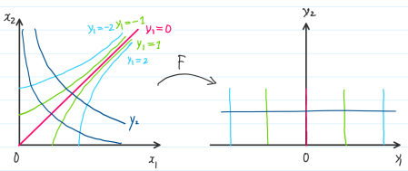
Example 2.5.3 Assuming $F : (0, + \infty) \times (0, + \infty) \to R \times (0, + \infty)$ where $(y_{1}, y_{2}) = F (x_{1}, x_{2}) = (x_{1}^{2} - x_{2}^{2}, 2 x_{1} x_{2})$ . Prove that $F$ is a diffeomorphism of $C^{\infty}$ . See Figure 2.5 for the contour plot.

2 2 == 4(x1 + x2) > 0

therefore $\partial F (x_{1}, x_{2})$ is invertible. Then $\begin{aligned} (x_{1}^{2} - x_{2}^{2}, 2 x_{1} x_{2}) & = (u_{1}^{2} - u_{2}^{2}, 2 u_{1} u_{2}) \\ (x_{1}^{2} + x_{2}^{2})^{2} & = (x_{1}^{2} - x_{2}^{2})^{2} + 4 x_{1}^{2} x_{2}^{2} \\ = (u_{1}^{2} - u_{2}^{2})^{2} + 4 u_{1}^{2} u_{2}^{2} = (u_{1}^{2} + u_{2}^{2})^{2} \\ \Rightarrow x_{1}^{2} \pm x_{2}^{2} = u_{1}^{2} \pm u_{2}^{2} \\ \Rightarrow x_{1}^{2} = u_{1}^{2}, x_{2}^{2} = u_{2}^{2} \\ \Rightarrow x_{1} = u_{1}, x_{2} = u_{2} \end{aligned}$

So $F$ is injective. Therefore, $F$ is a diffeomorphism.

Contour plot is very useful to visualize the correspondent relation, Figure 2.5 is another example.