Concavity and convexity

2.8 Concavity and convexity

Definition 2.8.1 $C \subseteq R^{n}$ is a convex if for any $x, y \in C$ , for any $0 \leq t \leq 1$ , $(1 - t) x + t y \in C$ .

Definition 2.8.2 $f : C \to R$ is a convex function if

$C$ is convex.
For any $x, y \in C$ , for any $0 \leq t \leq 1$ , $\begin{aligned} f ((1 - t) x + t y) \leq (1 - t) f (x) + t f (y) & (*) \end{aligned}$

Definition 2.8.3 $f$ is strictly convex if $f$ is convex and $(*)$ takes equality if and only if $x = y$ or $t = 0$ or $t = 1$ .

Definition 2.8.4 $f : C \to R$ is concave if $- f : C \to R$ is convex.

Definition 2.8.5 Assuming $f \in C^{2}$ , mark

∂2f Hf (x) == ∖lef t(-------∖right)n×n ∂xi∂xj

as the Hessian matrix of $f$ at $x$ .

Expand the Taylor series of degree

2

f \in C^{2}

x_{0}

, we have

\begin{aligned} f (x_{0} + v) & = f (x_{0}) + \sum_{i = 1}^{n} \frac{\partial f}{\partial x_{i}} (x_{0}) v_{i} + \underset{Quadratic form with respect to v}{\underset{⏟}{\frac{1}{2} \sum_{i, j = 1}^{n} \frac{\partial^{2} f}{\partial x_{i} \partial x_{j}} (x_{0}) v_{i} v_{j}}} + o (∥ v ∥^{2}) \\ = f (x_{0}) + \sum_{i = 1}^{n} \frac{\partial f}{\partial x_{i}} (x_{0}) v_{i} + \frac{1}{2} (\begin{array}{c} v_{1} & \dots & v_{n} \end{array}) {(\frac{\partial^{2} f}{\partial x_{i} \partial x_{j}})}_{n \times n} (\begin{array}{c} v_{1} \\ ⋮ \\ v_{n} \end{array}) \\ = f (x_{0}) + \sum_{i = 1}^{n} \frac{\partial f}{\partial x_{i}} (x_{0}) v_{i} + \frac{1}{2} v^{T} H_{f} (x) v \end{aligned}

Let $g (t) = f ((1 - t) x + t y)$ , $f \in C^{2} \Rightarrow g \in C^{2}$ . $f$ is (strictly) convex $\Leftrightarrow g$ is (strictly) convex on $[0, 1]$ . Therefore, for any $x \neq y$ , $\begin{aligned} g^{'} (t) & = \partial f ((1 - t) x + t y) (y - x) \\ = \sum_{i = 1}^{n} \frac{\partial f}{\partial x_{i}} ((1 - t) x + t y) (y_{i} - x_{i}) \\ g^{″} (t) & = \sum_{i, j = 1}^{n} \frac{\partial^{2} f}{\partial x_{i} \partial x_{j}} ((1 - t) x + t y) (y_{i} - x_{i}) (y_{j} - x_{j}) \\ = (y - x)^{T} H_{f} ((1 - t) x + t y) (y - x) \end{aligned}$

Terminally, we have

Theorem 2.8.6 Assuming $f \in C^{2}$ , for any $x$ , $\begin{aligned} H_{f} (x) is positive definite & \Rightarrow f is strictly convex \\ H_{f} (x) is semi-positive definite & \Leftrightarrow f is convex \\ H_{f} (x) is negative definite & \Rightarrow f is strictly concave \\ H_{f} (x) is semi-negative definite & \Leftrightarrow f is concave \end{aligned}$

Theorem 2.8.7 Assuming $f \in C^{2}$ is convex, then for any $x_{0}, x \in C$ ,

f(x) ≥ f (x ) + ∂f (x )(x − x ) 0 0 0

Definition 2.8.8 $x_{0}$ is a minimum point of $f$ , if there exists a neighborhood $u$ of $x_{0}$ such that for any $x \in U$ , $f (x) \geq f (x_{0})$ . If additionally $f (x) > f (x_{0})$ when $x \neq x_{0}$ , then $f$ is a strict minimum point. Similar for (strict) maximum point. Minimum points and maximum points are both extreme points.

Definition 2.8.9 $x_{0}$ is a critical point of $f$ if $\partial f (x_{0}) = 0$ , or for any $v \in {v \in R^{n} | ∥ v ∥ = 1}$ , $\frac{\partial f}{\partial v} = 0$ , or $\nabla f (x_{0}) = 0$ .

Theorem 2.8.10 (Fermat) Assuming $f$ is derivable at the extreme point $x_{0}$ , then $x_{0}$ is the critical point of $f$ .

Proof Assuming $\partial f (x_{0}) \neq 0$ , there exists $v \neq 0$ such that

-d- ∖lef t.dt f(x0 + tv)∖right|t=0 = ∂f(x0)(v) ⁄= 0

Assuming it to be positive, then there exists $δ > 0$ such that for any $- δ < t_{1} < 0 < t_{2} < δ$ ,

f(x0 + t1v) < f (x0 ) < f(x0 + t2v)

contradicted with that $x_{0}$ is the extreme point! $◻$

Theorem 2.8.11 Assuming $f \in C^{2}$ , $x_{0}$ is a critical point of $f$ . If $H_{f} (x_{0})$ is positive (negative) definite, then $x_{0}$ is the minimum (maximum) point of $f$ . If $H_{f} (x_{0})$ is not degenerate, yet it’s neither positive nor negative definite, then $x_{0}$ is a saddle critical point, not extreme point.

Example 2.8.1 Seek all extreme points for

f (x,y) =

View it in polar coordinate. $\begin{aligned} g (r, θ) & = r^{2} \cos θ \sin θ \ln r^{2} = r^{2} \ln r \sin 2 θ \\ \frac{\partial g}{\partial r} & = r (2 \ln r + 1) \sin 2 θ \\ \frac{\partial g}{\partial θ} & = 2 r^{2} \ln r \cos 2 θ \\ \frac{\partial^{2} g}{\partial r^{2}} & = (2 \ln r + 3) \sin 2 θ \\ \frac{\partial^{2} g}{\partial θ^{2}} & = - 4 r^{2} \ln r \sin 2 θ \\ \frac{\partial^{2} g}{\partial r \partial θ} & = 2 r (2 \ln r + 1) \cos 2 θ \end{aligned}$

Firstly,

⇔ r◟-=◝◜0 ◞ ∪∪ Abadoned

Left as exercise. :)

Example 2.8.2 Does

F (x, y,z) = x(1 + yz) + exp(x + y + z) − 1

determine a implicit function $z = f (x, y)$ near $(x, y, z) = (0, 0, 0)$ ? Expand the Taylor series of degree $3$ of $F (x, y, z)$ at $(0, 0, 0)$ to get $\begin{aligned} 0 & = x + x y z - 1 + (1 + z + \frac{1}{2} z^{2} + \frac{1}{6} z^{3} + o (z^{3})) \\ \cdot (1 + x + y + \frac{1}{2} (x + y)^{2} + \frac{1}{6} (x + y)^{3} + o ((x + y)^{3})) \\ = 2 x + y + z + \frac{1}{2} (x + y + z)^{2} + x y z + \frac{1}{6} (x + y + z)^{3} + \frac{(x + y)^{2} z^{2}}{4} + o ((x + y)^{3}) + o (z^{3}) \end{aligned}$

Assuming $r = \sqrt{x^{2} + y^{2}}$ , the linear part

2x + y + z = 0 ⇒ z = − 2x − y + o(z) + o(r)

so the linear equation has unique solution for any $(x, y)$ . According to IFT, there exists $z = f (x, y)$ near $(0, 0, 0)$ . Then it’s left as exercise. :)

Conditional extreme value. Target function

f (x_{1}, . . ., x_{n})

, constraining conditions

∖lef t{ ∖right.

See Figure 2.6 for instance.

Lagrange’s multiplier. Construct

F (x1,...,xn,λ1,...,λr) = f (x1, ...,xn ) − λ1g1 (x1,...,xn) − λrgr(x1,...,xn)

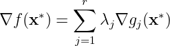
Theorem 2.8.12 Assuming $f, g_{1}, . . ., g_{r} \in C^{1}$ , $x^{*}$ is the (conditional) extreme point of $f$ under the condition $g_{1}, . . ., g_{r} = 0$ , then there exists $λ_{1}, . . ., λ_{r} \in R$ such that $(x^{*}, λ_{1}, . . ., λ_{r})$ is the critical point of $F$ , i.e.

\text{[math]}

As for (1), we have

∑ r ∇f (x∗) = λj∇gj (x∗) j=1

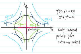
At $x^{*}$ , the level set (equal value set) of $f$ is tangent to the constrained surface $Σ = {x | g_{k} (x) = 0, k = 1, . . ., r}$ .

Theorem 2.8.13 Assuming $(x^{*}, λ^{*})$ is the critical point of $F$ , if the Hessian matrix $H$ of $F$ at $(x^{*}, λ^{*})$ is positive definite limited on the linear space $T_{x^{*}} Σ$ , i.e.

T v Hv > 0, ∀v ∈ Tx ∗ Σ ∖{0}

then $x^{*}$ is the strict minimum point of $f$ under the given constrained conditions. If $H$ is negative definite on $T_{x^{*}} Σ$ , then $x^{*}$ is the strict maximum point of $f$ under the given constrained conditions. If $H$ has either positive or negative eigenvalues on $T_{x^{*}} Σ$ , then $x^{*}$ is not the conditional extreme point of $f$ .

Example 2.8.3 Seek $(x y + y z + x z)_{min}$ when $x, y, z > 0$ and $x y z = 1$ . Construct

F(x, y,z,λ) = xy + yz + xz − λ(xyz − 1)

then we have

\text{[math]}

Notice that

λ = y-+-z-= x +-z-= x-+-y-⇒ x = y = z = 1,λ = 2 yz xz xy

The Hessian matrix

H =

$H$ is neither positive definite nor negative definite on $R^{3}$ , so we consider the constrained surface

Σ = {(x, y,z)|xyz = 1}, x∗ = (1,1,1)

The tangent space

T ∗ = ∖left{∖left.∖right|u + v + w = 1∖right} = ∖lef t{∖left.∖right |u, v ∈ ℝ∖right} x

Then the quadratic form

= 2(u2 + uv + v2) > 0

meaning $x^{*} = (1, 1, 1)$ is the conditional strictly minimum point of $f$ .

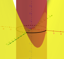
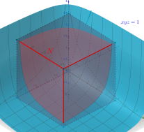
Yet does $f$ takes the minimum at $x^{*}$ ? (Counter-example showed in Example 2.8) See Figure 2.7 for hints.

If $x > N$ , then $y z = \frac{1}{x} < \frac{1}{N}$ , i.e. $y < \frac{1}{\sqrt{N}}$ or $z < \frac{1}{\sqrt{N}}$ . WLOG assuming $y < \frac{1}{\sqrt{N}}$ , then

1 √ --- f(x, y,z) ≥ xz = --> N > 3 ⇒ N > 9 y

Assuming $B = {(x, y, z) | x, y, z \in [0, 10]}$ , then for any $(x, y, z) \in (R^{+})^{3} ∖ B$ , $f (x, y, z) > 3 = f (1, 1, 1) \in B$ . Since $B \cap Σ$ is bounded closed, $f$ takes the minimum in $B \cap Σ$ , so $f$ take the minimum in $B$ . Terminally, $f$ takes the minimum at the conditional extreme point $(1, 1, 1)$ , and the conditional minimum of $f$ is $3$ .

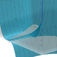
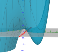
Example 2.8.4 Assuming $f : E \to R$ is derivable on $E \subseteq R^{m}$ , $x^{*}$ is the only critical point of $f$ and it’s a strict maximum(minimum) value, yet $f$ does not take the maximum/minimum at $x^{*}$ (even $f$ may be unbounded)! See Figure 2.8.

Figure 2.8: $z = e^{3 x} + y^{3} - 3 y e^{x}$